Sum of all Individual Probability Vectors equals General Vector
Just like QED, we say that summing up all the individual probability vectors creates the general Probability vector.
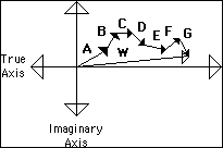
The Week vectors, W, are created by summing up the Day vectors, A -> G.
Week = S Days = Sum of Day Vectors
Similarly, summing up the Hour vectors creates the Day vectors, while summing up the Minute vectors creates the Hour vectors.
Day = S Hours
Hours = S Minutes

On the larger scale the Month vectors, M, are created by summing up the Weekly vectors, A -> D.
Month = S Weeks
Vectors represent Probabilities not Events
Remember from our past discussions that these vectors represent self-referential equations. They are each part of a Data Stream with its own Momentum. Hence while the general is the sum of the specifics - these are all average vectors - rather than the event itself. Thus the top graph could be expanded to look like this - with the actual events included in with the average.

The actual events, represented by the dotted vectors, are absorbed by the average vectors, (actually decaying average vectors, for they absorb the event and decay). Each event decays according to the same factors. Each event leaves a residue upon the decaying average. No event is ever lost once it has occurred. The impact of each event upon the average is proportional to its direction and how far away it is from the average - i.e. the distance away in events. From previously developed topics:
K = Scaling factor
D = Decay Factor > 1
K = (D-1)/D < 1
The impact of each event upon the average is reduced/scaled by how many events away from the average it is.
The point is that each event is absorbed by the decaying average of longer cycle as well as being the decaying average shorter cycle. As an example: the actual events that occur in seconds are the average of the millisecond, while they are the events upon which the minutes are based, which lay the foundation for hours, the days, weeks, months, years, decades, centuries, millennium, tens of thousands of years, millions, and then billions of years. Of course for Humans, the relevant Duration, i.e. the size of the time increment would probably be somewhere between minutes and decades. Under a minute is too short, while a century is too long. If humans were measured in centuries, we would all be either 1 or 0.
Totally irrelevant aside: Supposedly our Universe, our space-time continuum, is about 20 billion years old. If we live to 70 years old, we live about 2 billion seconds. Thus each second we live represents 10 years for our Universe.
Decay is relative - not absolute
Moving on. Because of the transitory nature of existence everything decays. However everything that has happened is contained as some type of remnant in the Present moment - leaving residual probability traces behind. The size of the traces is based upon the size of the Decay Factor, D. The larger the Decay factor the closer the Scaling factor, K, is to one. The larger the Scaling factor the less the Average Decays - hence the more stable it is. The relevant Decaying Average for a glacier makes humans look like a blink in time, while a relevant Decaying Average for a human makes the life cycle of a bug look trivial. The point is that there are no absolutes here, only relative truths.
We are merely reiterating issues contained more thoroughly in the book Data Stream Momentum. However, we are summarizing these issues as a foundation for a slightly different topic. Namely, QED is a representation of Human Reality. In similar fasihon, a picture is a representation of Reality, not Reality.
Four basic choices at any time
In our earlier analysis we suggested that there are two orthogonal/perpendicular universes that intersect, one the Real, the other the Imaginary. From these polarities we saw that in each moment Humans have four basic choices shown in the chart below.

The four choices are:
P(t) = Continue as normal
P(iF) = Veer off Path
P(iT) = Attempt to Return to Path
P(T) = On the Path
P(F) is actually just a component P(iF).
Each based in probabilities founded in past behavior
Further each of these choices have a probability associated with it based upon the vector/arrow, which sums up the past occurrences, after they’ve been appropriately scaled, of course. While each of the behaviors have distinct Probabilities with specific values and directions - in actuality there are an infinity of possible directions that behavior can take. However, in general P(iF) takes one away from the Path, while P(iT) brings one back to the Path. P(T) is the Path, while P(F) is opposite of the Path.
These are the polar parts of the real and imaginary world. While the Real, P(T), has only one Direction, which is Now, the Imaginary world of delusion by nature is infinite in variety. Similarly the Polluted, P(t), can point in any direction. While this Probability vector can point in any Direction, it only points in one direction at a time. If it points leftward into the second quadrant, we have renamed it P(f) to indicate that there is a higher probability of false behavior than true.
While True behavior, T, has only one direction, the probability of it occurring, P(T), is between 0% and 100%, from 0 to 1, just like any probability. Of course, only the hypothetical Guru is always in the Now, 100%. True Behavior, P(T) = 1 = P(t). However, most of us are more or less polluted, which means that we frequently respond emotionally and automatically to external situations. Each time we do this we raise the possibility of more false behavior in the future.
The point of this book is to give pointers as to how to raise the probability of being in the Now and lessen the probability of being emotionally distracted by desires and expectations of the future and regrets about the past. Changing behavior through intentionality based in investigation of underlying principles is a way to change these behavioral Probabilities.
Home The Firing Process V. Differentiation Previous Next Comments